Calculation of a Simple Feature
If you want to compute any of our features, you will first have to create a feature object. This is an object, which stores all the necessary information, such as the input data and control arguments.
The easiest way to create a feature object is to pass the arguments X and y to the function createFeatureObject, as illustrated in the example below.
library(flacco)

## (1) Generate some example data, i.e. create an initial sample 'X' consisting
## of 500 (2D) observations and compute the corresponding objective values 'y':
X = createInitialSample(n.obs = 500, dim = 2)
y = apply(X, 1, function(x) sum(sin(x) * x^2 + (x - 0.5)^3))

## (2) Create the corresponding feature object:
feat.object = createFeatureObject(X = X, y = y)

## (3) The feature object already contains some information on your data:
print(feat.object)

## (4) Calculate a feature set, e.g. the ELA meta model features:
calculateFeatureSet(feat.object, set = "ela_meta")
In order to find out, which feature sets can be computed, one could call the function listAvailableFeatureSets or have a look into the documentation of calculateFeatureSets. The latter one also contains a list of possible control options of each feature set.
Calculation of Expensive Features
Some feature sets (ELA convexity "ela_conv", ELA curvature "ela_curv" and ELA local search "ela_local") need to perform further function evaluations in order to compute the features. In those cases, it is necessary that the function (fun) is part of the feature object.
But don’t worry — if you don’t pass the function, calculateFeatureSet will complain and give you a hint.
Note, that it is also possible to pass only X and fun to createFeatureObject, i.e. you do not have to pass y. In that case, the objective values will be computed by createFeatureObject!
## (1) Create data
X = createInitialSample(n.obs = 2000, dim = 5)

## (2) Compute the feature object (note that we do not set any objective values)
feat.object = createFeatureObject(X = X, fun = function(x) sum(x^2))

## (3) Have a look at feat.object
print(feat.object)

## (4) Calculate the ELA convexity features
calculateFeatureSet(feat.object, set = "ela_conv")
Usually, you find more information on the parameters and thus on the exact number of additional function evaluations within the documentation of calculateFeatureSet. The following example shows you, how you could control the size of the generated sample:
## Calculate the convexity features using a sample of size 500,
## instead of the default of 1000.
calculateFeatureSet(feat.object, set = "ela_conv", control = list(ela_conv.nsample = 500))
A lot of our functions allow to configure certain details on how features should be computed using the control list parameter. However, as each function supports different parameters it is advisable to have a look into the corresponding documentation ?calculateFeatureSet.
Calculation of a Cell Mapping Feature
Cell mapping features differ from the others in the fact that they convert the continuous search space into a discretized one. This is achieved by dividing the entire search space into a grid with a finite amount of cells (per dimension). Each observation will then be assigned to exactly one cell. Afterwards, each cell will be represented by one (!) of its observations. So far, we provide 3 types of representatives of a cell. For further details, you should have a look into the pages of cell mapping and generalized cell mapping.
In order to define the grid, you need to specify the number of cells/blocks per dimension when creating a FeatureObject. If you don’t provide them, the attempt of computing a cell mapping feature will abort with an error.
## (1) Create data
X = createInitialSample(n.obs = 2000, dim = 5)
y = rowSums(X^2)

## (2) Compute a feature object
feat.object = createFeatureObject(X = X, y = y, blocks = c(10, 5, 5, 8, 4))

## (3) Have a look at feat.object
print(feat.object)

## (4) Calculate cell mapping features, e.g. the gradient homogeneity features
calculateFeatureSet(feat.object, set = "cm_grad")
The above example splits the data into 10 blocks in the first, 5 blocks in the second and third, 8 blocks in the fourth, and 4 blocks in the fifth dimension. If you always want the same amount of blocks in every dimension, you can even simplify your input:
## Compute the feature object
feat.object = createFeatureObject(X = X, y = y, blocks = 5)
Creating Explanatory Plots
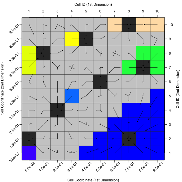
In addition to the features, the package provides plots, which visualize the features (or intermediate steps, which lead to the features). For example, the mechanics behind the generalized cell mapping approach are sometimes hard to grasp. In those cases, a plot, which visualizes the (two-dimensional) grid and indicates the transition probabilities from any cell to its attractor using proportional arrows, could be helpful. Such a plot can be created with the following commands (the corresponding plot is given below the R code).
library(smoof)
library(flacco)

## (1) Create data
X = expand.grid(seq(0, 1, length.out = 50), seq(0, 1, length.out = 50))
f = smoof::makeBBOBFunction(dimension = 2, fid = 17, iid = 9)
y = apply(X, 1, f)

## (2) Compute a feature object
feat.object = createFeatureObject(X = X, y = y, fun = f, blocks = c(10, 10))

## (3) Plot the corresponding cell mappings
plotCellMapping(feat.object, control = list(gcm.approach = "near"))
Similarly, the Barrier Tree usually become more clear, when visualizing them. flacco allows its users to create 2D and 3D barrier trees. The former one look similar to the aforementioned cellmappings - extended by the branches of the tree.
## (a) a 2D plot of the barrier trees
plotBarrierTree2D(feat.object, control = list(gcm.approach = "near", bt.cm_surface = FALSE))

## (b) based on a combination of the R function 'persp' and the barrier tree
## approach, one now can produce 3D plots of the barrier trees
ctrl = list(gcm.approach = "near", bt.persp_border = "lightgrey",
  bt.persp_theta = 35, bt.persp_phi = 25, bt.color_surface = "pink",
  bt.persp_shade = 0.1, bt.persp_ticktype = "simple",
  bt.persp_xlab = "x", bt.persp_ylab = "y", bt.persp_zlab = "f(x, y)")
plotBarrierTree3D(feat.object, control = ctrl)


Please note, that the barrier tree features currently only work for problems with a 2D decision space. If you try to compute them for higher dimensional problems, you will receive an error.
Compute all Feature Sets at Once
In case you have a feature object, which is a discretized version of a 2D input space and which provides the original function as well, you can compute all available feature sets at once — using calculateFeatures.
X = createInitialSample(n.obs = 1000, dim = 2)
f = function(x) sum(x^3 * sin(x))
feat.object = createFeatureObject(X = X, fun = f, blocks = 5)
features = calculateFeatures(feat.object)