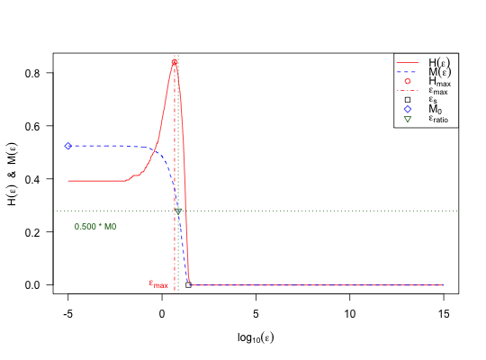
Plot Information Content
Creates a plot of the Information Content Features.
plotInformationContent(feat.object, control)
Arguments
| feat.object | [ |
|---|---|
| control | [ |
Value
[plot].
A plot visualizing the Information Content Features.
Details
Possible control arguments are:
Computation of Information Content Features:
ic.epsilon: Epsilon values as described in section V.A of Munoz et al. (2015). The default isc(0, 10^(seq(-5, 15, length.out = 1000)).ic.sorting: Sorting strategy, which is used to define the tour through the landscape. Possible values are"nn"(= default) and"random".ic.sample.generate: Should the initial design be created using a LHS? The default isFALSE, i.e. the initial design from the feature object will be used.ic.sample.dimensions: Dimensions of the initial sample, if created using a LHS. The default isfeat.object$dimension.ic.sample.size: Size of the initial sample, if created using a LHS. The default is100 * feat.object$dimension.ic.sample.lower: Lower bounds of the initial sample, if created with a LHS. The default is100 * feat.object$lower.ic.sample.upper: Upper bounds of the initial sample, if created with a LHS. The default is100 * feat.object$upper.ic.show_warnings: Should warnings be shown, when possible duplicates are removed? The default isFALSE.ic.seed: Possible seed, which can be used for making your experiments reproducable. Per default, a random number will be drawn as seed.ic.nn.start: Which observation should be used as starting value, when exploring the landscape with the nearest neighbour approach. The default is a randomly chosen integer value.ic.nn.neighborhood: In order to provide a fast computation of the features, we useRANN::nn2for computing the nearest neighbors of an observation. Per default, we consider the20Lclosest neighbors for finding the nearest not-yet-visited observation. If all of those neighbors have been visited already, we compute the distances to the remaining points separately.ic.settling_sensitivity: Threshold, which should be used for computing the “settling sensitivity”. The default is0.05(as used in the corresponding paper).ic.info_sensitivity: Portion of partial information sensitivity. The default is0.5(as used in the paper).
Plot Control:
ic.plot.{xlim, ylim, las, xlab, ylab}: Settings of the plot in general, cf.plot.default.ic.plot.{xlab_line, ylab_line}: Position ofxlabandylab.ic.plot.ic.{lty, pch, cex, pch_col}: Type, width and colour of the line visualizing the “Information Content” \(H(\epsilon)\).ic.plot.max_ic.{lty, pch, lwd, cex, line_col, pch_col}: Type, size and colour of the line and point referring to the “Maximum Information Content” \(H[max]\).ic.plot.settl_sens.{pch, cex, col}: Type, size and colour of the point referring to the “Settling Sensitivity” \(\epsilon[s]\).ic.plot.partial_ic: Should the information of the partial information content be plotted as well? The default isTRUE.ic.plot.partial_ic.{lty, pch, lwd, cex, line_col, pch_col}: Type, size and colour of the line and point referring to the “Initial Partial Information” \(M[0]\) and the “Partial Information Content” \(M(\epsilon)\).ic.plot.half_partial.{pch, cex, pch_col}: Type, size and colour of the point referring to the “Relative Partial Information Sensitivity” \(\epsilon[ratio]\).ic.plot.half_partial.{lty, line_col, lwd}_{h, v}: Type, colour and width of the horizontal and vertical lines referring to the “Relative Partial Information Sensitivity” \(\epsilon[ratio]\).ic.plot.half_partial.text_{cex, col}: Size and colour of the text at the horizontal line of the “Relative Partial Information Sensitivity” \(\epsilon[ratio]\).ic.plot.legend_{descr, points, lines, location}: Description, points, lines and location of the legend.
References
Munoz, M. A., Kirley, M., and Halgamuge, S. K. (2015): “Exploratory Landscape Analysis of Continuous Space Optimization Problems Using Information Content”, in: IEEE Transactions on Evolutionary Computation (19:1), pp. 74-87 (http://dx.doi.org/10.1109/TEVC.2014.2302006).
Examples
# (1) create a feature object:
X = t(replicate(n = 2000, expr = runif(n = 5, min = -10, max = 10)))
feat.object = createFeatureObject(X = X, fun = function(x) sum(x^2))

# (2) plot its information content features:
plotInformationContent(feat.object)