Plot Cell Mapping
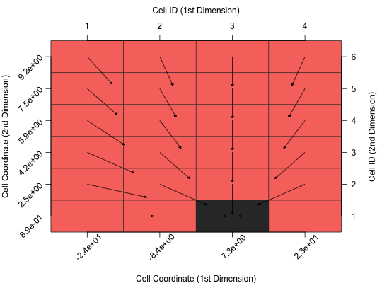
Visualizes the transitions among the cells in the General Cell Mapping approach.
plotCellMapping(feat.object, control)
Arguments
| feat.object | [ |
|---|---|
| control | [ |
Value
[plot].
Details
Possible control arguments are:
Computation of GCM Features:
gcm.approach: Which approach should be used when computing the representatives of a cell. The default is"min", i.e. the observation with the best (minimum) value within per cell.gcm.cf_power: Theoretically, we need to compute the canonical form to the power of infinity. However, we use this value as approximation of infinity. The default is256.
Plot Control:
gcm.margin: The margins of the plot as used bypar("mar"). The default isc(5, 5, 4, 4).gcm.color_attractor: Color of the attractors. The default is"#333333", i.e. dark grey.gcm.color_uncertain: Color of the uncertain cells. The default is"#cccccc", i.e. grey.gcm.color_basin: Color of the basins of attraction. This has to be a function, which computes the colors, depending on the number of attractors. The default is the color scheme fromggplot2.gcm.plot_arrows: Should arrows be plotted? The default isTRUE.gcm.arrow.length_{x, y}: Scaling factor of the arrow length in x- and y-direction. The default is0.9, i.e. 90% of the actual length.gcm.arrowhead.{length, width}: Scaling factor for the width and length of the arrowhead. Per default (0.1) the arrowhead is 10% of the length of the original arrow.gcm.arrowhead.type: Type of the arrowhead. Possible options are"simple","curved","triangle"(default),"circle","ellipse"and"T".gcm.color_grid: Color of the grid lines. The default is"#333333", i.e. dark grey.gcm.label.{x, y}_coord: Label of the x-/y-coordinate (below / left side of the plot).gcm.label.{x, y}_id: Label of the x-/y-cell ID (above / right side of the plot).gcm.plot_{coord, id}_labels: Should the coordinate (bottom and left) / ID (top and right) labels be plotted? The default isTRUE.
References
Kerschke, P., Preuss, M., Hernandez, C., Schuetze, O., Sun, J.-Q., Grimme, C., Rudolph, G., Bischl, B., and Trautmann, H. (2014): “Cell Mapping Techniques for Exploratory Landscape Analysis”, in: EVOLVE -- A Bridge between Probability, Set Oriented Numerics, and Evolutionary Computation V, pp. 115-131 (http://dx.doi.org/10.1007/978-3-319-07494-8_9).
Examples
# (1) Define a function: library(smoof)#>#>#>#> Warning: package ‘checkmate’ was built under R version 3.4.1f = makeHosakiFunction() # (2) Create a feature object: X = cbind( x1 = runif(n = 100, min = -32, max = 32), x2 = runif(n = 100, min = 0, max = 10) ) y = apply(X, 1, f) feat.object = createFeatureObject(X = X, y = y, blocks = c(4, 6)) # (3) Plot the cell mapping: plotCellMapping(feat.object)
